FiNTA · Filament Network Tracing Algorithm
Measuring fibre networks.
FiNTA traces every single fibre of a network and turns the picture into numbers: fibre lengths, orientations, mesh sizes, persistence lengths. Where the image came from is all the same to the algorithm — electron microscopy, fluorescence, confocal, brightfield, AFM: visible fibres are enough. Bitblade Group has made the published algorithm accessible as a web interface, together with the FiNTA team — upload an image, measure the fibre thickness, download the result as a report or as raw data.
EXAMPLE RUN
A complete run to take home
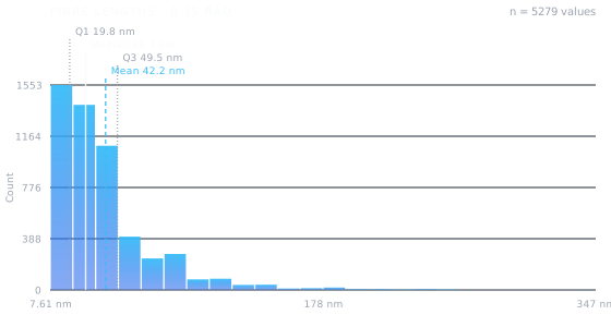
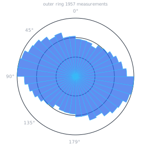
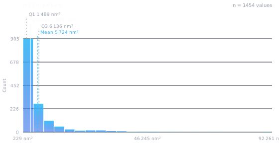
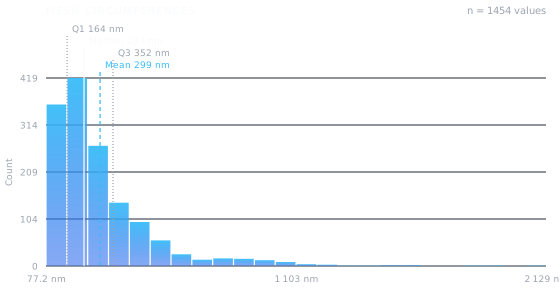
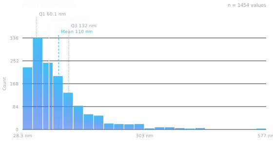
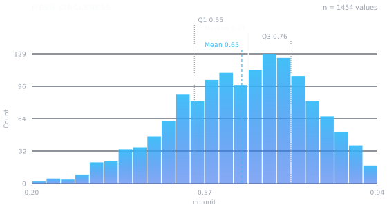
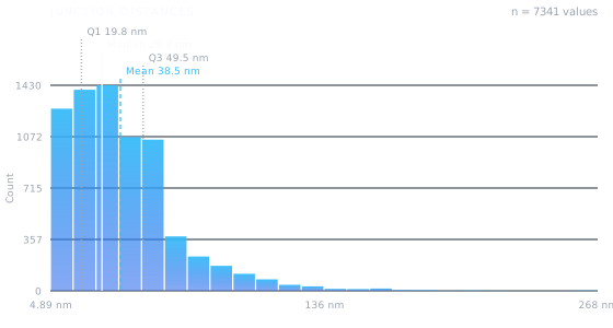
Computed on the micrograph from the cell nucleus further down — with exactly the settings the clip there is based on. The seven charts are drawn from the extracted data.
metrics.json and the log of the
run.
ZIP · 40 MB · 26 files — 33 MB of that the recording
A scale is set according to the scale bar.
BEFORE / AFTER
The same spot, before and after
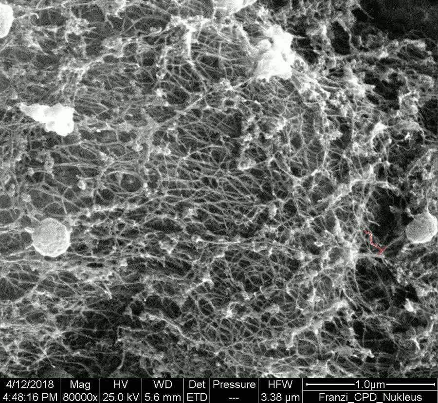
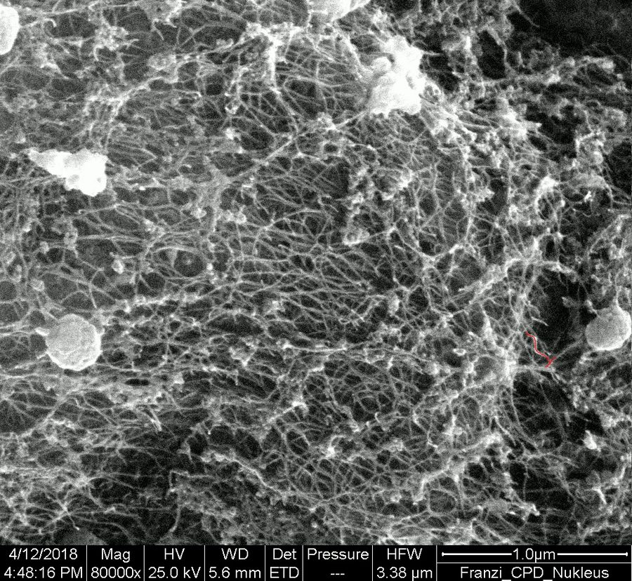
On the left the micrograph as it came out of the electron microscope. Drag the edge.
 IMAGE
IMAGE
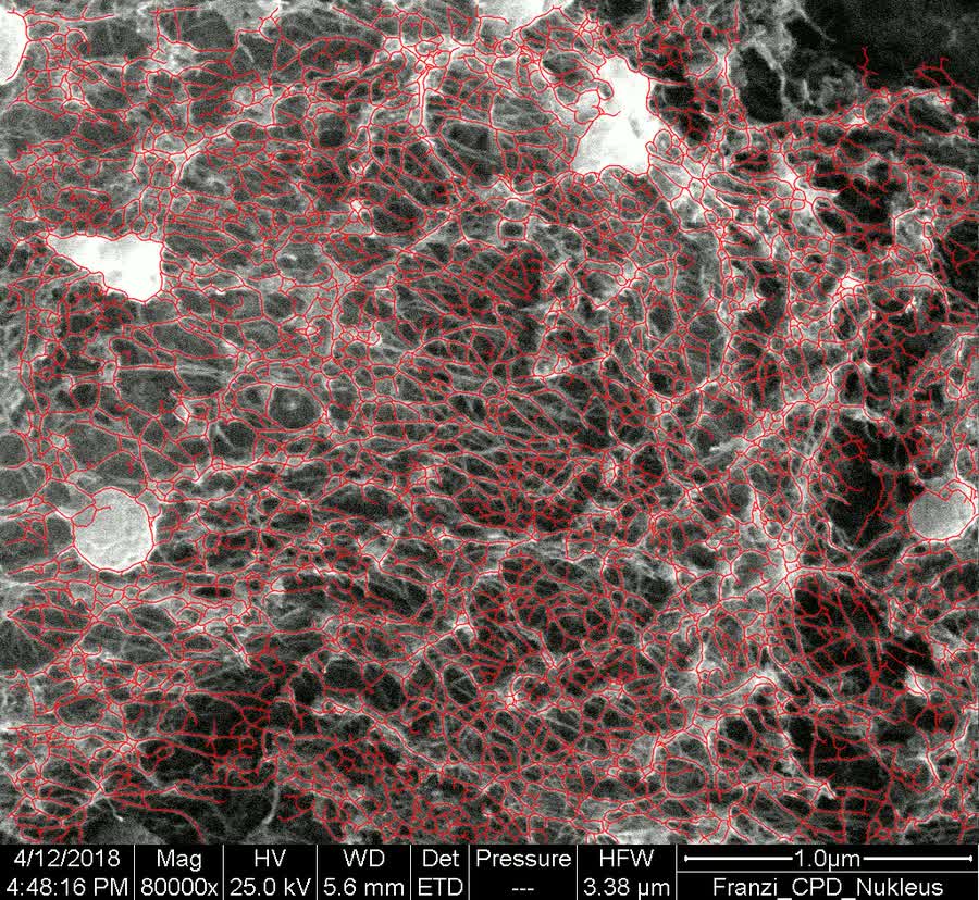 AFTER 536 ITERATIONS
The image shows actin fibres of the actin cortex above the nucleus. Fibre diameter set to 4 pixels for this run, threshold 1.3 · 536 iterations. The annotations at the bottom of the image are excluded from the tracing.
WORKFLOW
From image to analysis
Upload an image
Any image in which the individual fibres can be made out. Greyscale or colour — colour images are converted to greyscale internally, or you deliberately trace a single colour channel.
Measure the fibre thickness
Drag once across a fibre in the image. Good tracing parameters can be guessed from this number; getting it right is essential for good results.
A drag along the scale bar additionally sets the image scale — after that every result comes in real units instead of pixels.
Run the tracing
The run executes as a background job against the original compiled FiNTA binary, not against a reimplementation. On request it records every tracing iteration as a frame along the way.
Analyse and export
Charts and key figures straight in the browser, plus a PDF report and a ZIP holding every artefact, the log, the settings file used and the numbers as CSV — both of them here to download.
CHOICE OF CHANNEL
One image, two answers
Three pairs, each from a single image: left and right show the same picture, only the colour channel analysed is a different one. What ends up being measured is decided here. The colour of the lines, by the way, is freely selectable and says nothing about the channel.
The nuclei sit on the blue channel. The algorithm promptly finds their rims — cleanly and completely. It shows that FiNTA, while built for fibre analysis, can be used for other things too.
The same picture, red channel: now the tracing runs through the fibre work of the whole cell.
Green channel: actin fibres.
Red: vimentin fibres.
TRACING
Watching the fibres being found
Seven runs on scanning electron micrographs, one frame per tracing iteration. The red is always the same: the centre lines the algorithm has found up to that frame. The same recording is produced for any run of your own, if the animation is switched on.
All six images come from the work of the FiNTA team. The values shown in them were written into the picture by the instrument; the parameter values are taken from the settings file each run was computed with. All clips are silent and carry no audio track whatsoever.
NO INSTRUMENT REQUIRED
It does not have to be a microscope.
No sample preparation, no instrument — a night photograph taken with a camera, and the same algorithm draws the same centrelines, here in blue instead of red. What FiNTA asks for is not a particular imaging technique, but fibres that stand out from the background.
CONTROL CASES
Three images that are not a measurement series
They show no result but the method: what happens when you put something in front of it whose answer you already know — and what happens when fibres lie black on a light ground instead of light on a dark one.
The simplest touchstone
A regular grid, photographed at an angle. Here you know beforehand what has to come out: straight lines, equal spacings, right angles — and you see at once whether the chosen settings are any good.
Dark fibres, light ground
The algorithm looks for bright ridges. Branches against the sky are the opposite — so the image is inverted before the run. A setting, not a special case.
The whole run, uncut
Over a thousand iterations on a weeping birch, started from two points set by hand rather than automatically. Long enough to see how the tracing first takes hold of the trunk, then the strong branches, and last of all the fine mesh at the edge of the crown.
The line colour is a setting
Here the same algorithm draws in blue — because it shows up better over the warm sparks. Red is merely the most frequent choice on this page, not a property of the method.
MEASURED QUANTITIES
The data which you can extract
Every distribution comes as a chart, as a table and as a raw file.
Fibre lengths
Distribution across the entire network, optionally across only those fibres that bound closed meshes. The intersection angle at which a new fibre begins at a junction is adjustable. See the example.
Orientations as a rose diagram
A fibre has no head and no tail, which is why FiNTA folds every connection into [0°, 180°). On a linear axis 179° and 1° would sit at opposite ends, although they are very nearly parallel. For the same reason the rose carries no mean, no median and no preferred direction. See the example.
Persistence length
For the network as a whole, as in the paper — and per fibre on top of that, plotted against the fibre length. In the example run it comes to 524 nm for the network as a whole.
Meshes and junctions
Areas, circumferences and diameters of the closed meshes, along with the distances between junction points. See the example.
Density map
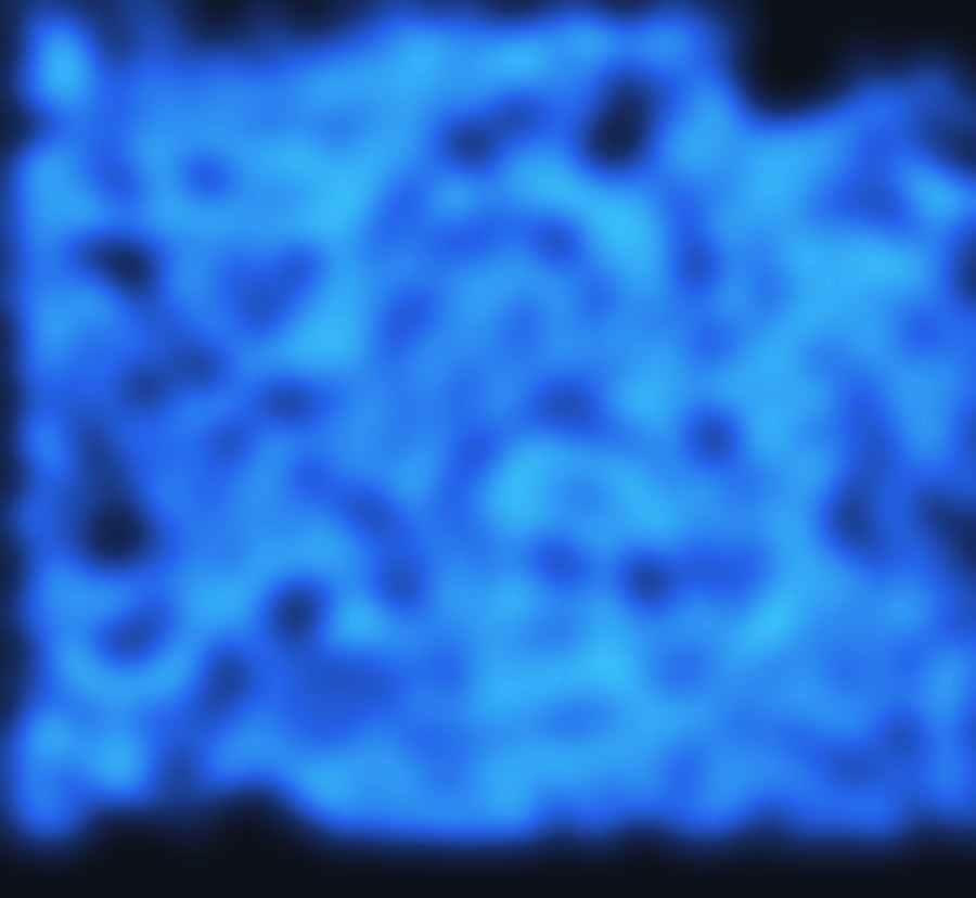
The one question no average answers: where in the picture the network actually lies. With adjustable smoothing and a colour scale that follows the smoothing.
Animation of the tracing
One frame per tracing iteration, transcoded to H.264 and playable straight in the job view. Useful for seeing where a tracing breaks off or cuts a curve short — the examples further up are exactly such recordings.
PUBLICATION
The algorithm is published — and citable
The algorithm is not ours; it comes from the authors named below. Once the publication was complete, Bitblade Group built this web interface together with the FiNTA team — so that researchers and everyone else with an interest can use the software by an easy route, without compiling it themselves, without a command line and without a compute environment of their own. The computing is done unchanged with the method from that work.
Flormann DAD, Schu M, Terriac E, Thalla D, Kainka L, Koch M, Gad AKB, Lautenschläger F. A novel universal algorithm for filament network tracing and cytoskeleton analysis. FASEB J. 2021 May;35(5):e21582. doi: 10.1096/fj.202100048R. PMID: 33835502.
To the publication (DOI) On PubMed Source code on GitHubCitation in the export
Every PDF report produced carries the full reference on every page.
THE TEAM BEHIND THE ALGORITHM
Authors
Developed at Saarland University and at the INM – Leibniz Institute for New Materials, Saarbrücken, with contributions from Sheffield and Funchal. The algorithm itself was written and developed by Moritz Schu; what the others contributed is stated next to their names and follows the contribution statement of the publication.
Affiliations as given in the publication. FiNTA is licensed under the GNU General Public License v3.0; this web interface changes nothing about that.
ACCESS
Get started
You create an account, upload your image and start the first run — no installation, no command line. The application is built for separate tenants: the images, runs and results of one workspace are neither visible nor addressable from any other.
Create an account Ask a question
What happens when you sign up. You give a name and an email address, confirm the address through a link we send you, and you have a workspace only you can see. Anyone working on the same data as a group gets a shared workspace on top — that is decided by group membership in the sign-in service, and by nothing anybody could type into a browser. Which data this produces is set out in the privacy notice.
 IMAGE
IMAGE
 CENTRELINES
 DENSITY